Scraping and Mapping North Dakota Rig Counts with R

I created a PDF knitr version of this post if you’d like to view that instead.

Intro

Rig count data can be found at Baker Hughes’ website. However, some state regulators have readily available rig count data. North Dakota is one such state. In this post, I am going to briefly go over how we can scrape the North Dakota rig count table, aggregate that data, and map that aggregated data.

Scraping

First, we need to load dependencies, set a variable to record the date which we are scraping the data, read the url, and then parse the html page for some necessary nodes to create filters (so that you can find the table you are looking for.

# Scrape and Build List ---------------------------------------------------

### Load Dependencies
    library(rvest)

### Create variable for map header and file name if you so choose to save this data
    today <- Sys.Date()

### Load URL and scrape tables and table attributes
    ### Create URL, load URL, scrape all table nodes, scrape all table attributes = "summary"
        url           <- "https://www.dmr.nd.gov/oilgas/riglist.asp"
        html          <- url %>% read_html()
        table         <- html %>% html_nodes("table")
        table.summary <- table %>% html_attr("summary")

Now that we have the html content plus the nodes, we can filter to find the table. We will more than likely want to use the “summary” attribute value “results” to filter the table with all the rig count information. After that, we will want to extract the table, extract the headers (because they don’t come with the table in this case), and put it all together.

### Build table attributes filter and subset list of tables on that
    ### Create a filter to find the correct table, subset the table nodes with that filter, and extract the table
        table.filter <- grep("results", table.summary)
        rig.table    <- table[table.filter] %>% html_table()

    ### Extract the table from the list, find the header, and apply the header to the table
        rig.table           <- rig.table[[1]]
        rig.table.header    <- table[table.filter] %>%
                               html_nodes("thead") %>%
                               html_nodes("th") %>%
                               html_text()
        colnames(rig.table) <- rig.table.header

Now let’s preview the data.

### Preview the table
    head(rig.table[c(1:3,5)])

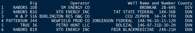
Looks great. Now let’s map it.

Mapping prep work: getting the county data

We’ll use “choroplethr” to map the rig count information at the county level. So first thing to do is load all the dependencies.

# Map the Data ------------------------------------------------------------

### Load Dependencies
    library(ggplot2)
    library(choroplethr)
    library(choroplethrMaps)
    library(plyr)
    library(dplyr)
    data("county.regions")

Next thing we need to do is fetch the county names – because in the preview above all we have are abbreviations. We’ll load in an html session using “rvest”, parse the forms in the session, set values for our form, and submit that form.

### Oil & Gas Code Definitions
    ### Submit form and get new session
        url         <- "https://www.dmr.nd.gov/oilgas/codehelp.asp"
        session     <- url %>% html_session()
        form        <- session %>% html_form()
        form.values <- form[[1]] %>% set_values(SELECTCODE = "County API")
        new.session <- session %>% submit_form(form.values, submit = "B1")

Now that we have the new session, we are going to parse out the table we are looking for (which is the 2nd table in the list), and then we are going to give it some custom header information. Then I am going to create an “Abbreviation” column similar to what the rig table has (to merge/join on in a few steps), and reduce all “CountyName” values to lower case (to merge/join in the next step).

    ### Parse new session for table
        table               <- new.session %>% html_nodes("table")
        counties.raw        <- table[[2]] %>% html_table()
        names(counties.raw) <- c("Code", "CountyName")
        counties.raw        <- counties.raw %>%
                               mutate(Abbreviation = substr(counties.raw$CountyName,
                                                            start = 1,
                                                            stop = 3))
        counties.raw$CountyName <- counties.raw$CountyName %>% tolower()

Now we can merge/join that information with the “choroplethrMaps” data so that “choroplethr” can search by the “region” associated with each county.

    ### County Regions
        regions   <- filter(county.regions, state.name == "north dakota") %>%
                     select(region, "CountyName" = county.name)

    ### Merge
        counties <- merge(counties.raw, regions, by = "CountyName")

Mapping prep: aggregating and creating the “value” column

We now need to do the R-equivalent of a “GROUP BY” statement for each county (we’ll use “Abbreviation” as the column to merge/join on). We want to county the number of rigs in each county, so we will use “aggregate” and then merge/join that data with the one above which has all the “region” values for each county. Then we need to add a new column, “value”, so that “choroplethr” knows what to map. We will assign “RigCount” values to “value” (we are going to copy the rig counts to “values”).

### Begin aggregation, merging, and mapping
    ### Lazy aggregation
        rig.county.list <- aggregate(. ~ County, data = rig.table, FUN = length) %>%
                           select("Abbreviation" = County, "RigCount" = Rig)

    ### Merge
        rig.county.list <- merge(rig.county.list, counties, by = "Abbreviation")

    ### Map/Save prep
        map.title             <- paste("North Dakota Rig Count \n", today)
        rig.county.list$value <- rig.county.list$RigCount
        num.colors            <- dim(rig.county.list)[1] + 1

    ### Map
        choro_rigs <- county_choropleth(rig.county.list,
					state_zoom = "north dakota",
					legend = "Count",
					num_colors = num.colors) +
                      ggtitle(map.title) +
                      coord_map()  # Adds a Mercator projection

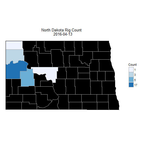
Now let’s take a look at the results of this work.

    ### View the map
        choro_rigs